|
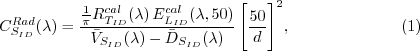
|
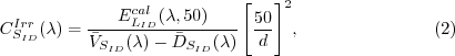
|
|
| Radiometers
calibration & characterization |
| Characterization and calibration
of field radiometers are crucial elements of a calibration/validation
program for ocean color remote sensing satellites.
The activities performed in this segment are outlined
in the following subsections: Calibration, Stability, Immersion
coefficient, and Bio-fouling. |
| Radiometers:
Calibration |
The
absolute calibration of the SPMR and SMSR with respect
to NIST-traceable standards is performed every six
months in the Satlantic optics calibration laboratory.
The aim of the absolute calibrations is to find a
coefficient for each sensor to relate the raw instrument
counts measured in an environment to the actual quantity
of the parameter being measured in that environment.
The method for doing this for radiance and irradiance
sensors varies slightly and has been documented by
Hooker et al. (2002).
For a radiance sensor (identified by  ),
the calibration coefficient is computed using a plaque
(identified by ),
the calibration coefficient is computed using a plaque
(identified by  )
with a calibrated reflectance, )
with a calibrated reflectance,  along
with a standard lamp (identified by )
that has a calibrated irradiance, along
with a standard lamp (identified by )
that has a calibrated irradiance,  .
As a general procedure, the lamp is required to be
positioned on axis and normal to the center of the
plaque at a distance d. Dark digital voltage
levels are recorded with the radiance sensor capped
and an average dark level, .
As a general procedure, the lamp is required to be
positioned on axis and normal to the center of the
plaque at a distance d. Dark digital voltage
levels are recorded with the radiance sensor capped
and an average dark level,  ,
is taken from these dark samples. ,
is taken from these dark samples.
The radiance sensor position allows a 45o view
of the plaque with respect to the lamp illumination
axis. Once the lamp is powered on, the voltage levels
of each of the individual sensor channels are recorded.
From these, an average calibration voltage for each
channel,  ,
is obtained. The calibration coefficient is calculated
as: ,
is obtained. The calibration coefficient is calculated
as:
where, d is given in centimeters.
For an irradiance sensor (identified by SID), the
calibration coefficients are computed using an FEL
standard lamp ( )
with a calibrated irradiance cal )
with a calibrated irradiance cal  .
As a general procedure the lamp is required to be
on axis and normal to the face plate of the irradiance
sensor at a distance, d. Similar to the
radiance sensor, dark voltage levels (digital) are
recorded with the radiance sensor capped and an average
dark level, ,
is taken from these dark samples. .
As a general procedure the lamp is required to be
on axis and normal to the face plate of the irradiance
sensor at a distance, d. Similar to the
radiance sensor, dark voltage levels (digital) are
recorded with the radiance sensor capped and an average
dark level, ,
is taken from these dark samples.
With the lamp powered on, the voltage levels of
each of the individual sensor channels are recorded.
From these, an average calibration voltage for each
channel, ,
is obtained. The calibration coefficient is calculated
as:
where, d is given in centimeters.
Back
to top |
| Radiometers:
Stability |
The
methodology and equipment used for tracking the stability
of our main field radiometers are now sketched out
in the following three subsections.
Radiometer
stability: The SQM-II
The SQM-II is a portable stable light source
originally designed under the name SQM, standing
for SeaWIFS Quality Monitor, by NASA and NIST (Johnson
et al. 1998). The SQM-II has been redesigned and
built by Satlantic, Inc. The SQM-II consists of a
lamp housing and a power box, which are connected
by a 5m cable. A serial port provides the capability
of monitoring and controlling the system with a PC.
An internal memory, an LCD display, and several buttons
on the back also allow manual control and monitoring.
Several status LEDs are also used to provide a quick
method for determining the state of the instrument.
The SQM-II has two sets of eight bulbs each. There
is no individual bulb control, a set is either completely
turned on or off. The light output of the second
set, called the high power bank, is about three times
brighter than the light output of the first set,
named the low power bank. They are often referred
to as HiBank and LoBank respectively. These two lamp
banks provide three illumination levels: low illumination
when only LoBank is on, medium illumination when
only HiBank is on, and high illumination when both
lamp banks are on.
A sensitive internal detector at 490 nm is used
to monitor the stability of the lamps. The outputs
from this detector and other internal sensors measuring
temperatures, voltages and currents are monitored
by a 20-bit analog-to-digital converter.
The SQM-II setup is precisely described in the
SQM-II user's manual edited by Satlantic.
Back
to top
Radiometer
stability: Methodology
To check the stability of the different radiometers in the field and to monitor
the performance of the SQM-II itself, a calibration evaluation and radiometric
testing (CERT) session and a data acquisition sequence (DAS) have been defined
following the procedure described in Mueller et al. (2002). A CERT session
is a sequence of DAS events, which are executed following a prescribed methodology.
Each DAS lasts for 3min to represent enough data to statistically establish
the characteristics of the instrument involved referred to as DUT, standing
for Device Under Test. This records about 1,000 DUT records and 450 SQM-II
records. A typical sequence of procedures for each CERT session is as follows:
- The electronics equipment (lamp power supplies,
the SQM-II fan and internal heater power supplies,
lamp timers, etc.) is turned on at least 1 hour
before the CERT session begins. The total number
of hours on each lamp set are tracked by recording
the starting and the ending of hours on each lamp
set. Each lamp bank acts as a separate state machine.
The state of a given lamp bank is independent of
the state of the other bank.
- The SQM-II lamp bank will remain in this coarse
stability state for 1h, allowing enough time for
the lamp and the system to thermally stabilize.
It is not recommended that radiometer measurements
be taken while in this state since the lamps have
not yet reached their highest stability. After
one hour, the lamp banks will automatically enter
the fine stability state.
- If the mixture of radiometers used in the CERT
session changes over time, at least one radiometer
(preferably two of different types, i.e. radiance
and irradiance) should be used in all CERT sessions.
This would be practically the case when the SPMR
system and the buoy radiometers are not calibrated
during the same CERT.
- S. Hooker advises to keep the banks in the fine
stability state for another hour before starting
the CERT, particularly in highly variable environments.
This advice was followed so far even if the CERT
took place in a laboratory. The warm-up period
can be considered completed when the internal SQM-II
monitor data are constant within 0.1%. The radiometric
stability usually coincides with a thermal equilibrium
as denoted by the internal thermistors.
- The insertion of a DUT into the shadow collar
of the SQM-II light chamber has a small loading
effect on the SQM-II due to its reflectivity, i.e.,
some light reflected back into the light chamber.
This in turn affects what the radiometer sees.
However the reflectivity of a field radiometer
is constantly changing over time due to the normal
wear and tear of use, altering the loading effect
on the SQM-II monitor detector and the effective
light field seen by the radiometer.
- Hence, upon the completion of the warm-up period,
SQM-II monitor data are collected for the black
glass (radiance) and white (irradiance) fiducials
successively. A fiducial is a non-functional DUT,
whose reflective surface must be carefully maintained
over time so that its reflectivity remains essentially
constant. It is also important that the position
of the fiducial in the compartment is always the
same and this is ensured by a fixed collar allowing
only one position.
- Once these control measurements are completed,
the individual radiometers (DUTs) are then tested
sequentially. This begins with an 1=OCR-2001 that
is designated specifically for use on the SQM-II
and nothing else. Its use is restricted solely
to SQM-II sessions to preserve the performance
of its original calibration and, hence, serve as
a verification of SQM-II stability between sessions.
- Firstly, the DUT sensor head is inserted and
secured in the SQM-II compartment. Data is collected
over 3min. The DUT is secured using the three fasteners
on the SQM-II which clamp on a collar that has
been fastened to the DUT. This collar is at a specific
distance from the sensor head and of a particular
rotational position, determined by the flat side
of the collar. This positioning of the flat part
of the collar ensures that the DUT always enters
the SQM-II in exactly the same way.
- The DUT is removed from the SQM-II slot and the
caps are placed over the sensor heads to block
out all possible light to the them. The black fiducial
is then placed in the 1=SQM-II1 and data is again
collected from both 1=SQM-II1 and DUT to provide
a dark reading for the DUT and stability check
for the 1=SQM-II1 . Each time any file is recorded,
the voltage at the SQM-II internal detector is
noted.
- Once all instruments have been tested, SQM-II
monitor data are collected a second time for black,
radiance and irradiance fiducials successively.
- As soon as all measurements with a lamp bank
are complete and its use is no longer required,
the lamps are switched off to minimize aging and
possible deteriation. Where an alternative lamp
bank combination is required for testing DUTs at
a different light intensity, 2h warm-up time is
once again required to reach optimum stability.
- The use of all three light intensity levels (Lo,
Medium and Hi-Bank) was discontinued in 2003 because
changes in SQM-II performance causing saturation
of the internal detector of the SQM-II during Hi-Bank
operation have led to the omittance of Hi-Bank
measurements.
- Before the SQM-II is finally shut down and the
CERT session completed, after the lamps are powered
down, the ending number of hours on each lamp set
is recorded.
The SQM-II operation
is precisely described step by step in the SQM-II
User's Manual edited by Satlantic, although some
changes have been made to our method to reduce the
duration of each SQM-II session and to accommodate
the aforementioned internal detector saturation during
Hi-Bank operation.
Back
to top
Radiometer
stability: Measurement schedule
The objective of the scheduling of the SQM-II operations is to arbitrarily
monitor variability and drift of the optics sensors during the period of use
between the near-biannual absolute calibrations which are performed by Satlantic
at their Halifax, Nova Scotia facility. The data collected in these SQM-II
sessions aids in the reduction of error in the field data caused by changes
in the performance of the sensors between the times of absolute calibrations.
When differences occur between these calibrations, it cannot be assumed that
this change has been a gradual and linear process during the period of activity.
As soon as possible
after the radiometers are received in Villefranche
after shipment by Satlantic from the absolute calibration
in Canada, they are tested on the SQM-II in the optics
laboratory in Villefranche, using the method described
in section 6.2.2.
Once the sensors have
been active in the field, either fixed on the buoy
or profiled from the ship, they are once again subjected
to testing on the SQM-II. The exact scheduling of
this testing depends upon the duration of their activity.
For the buoy radiometer heads, which are intended
to be exchanged on a monthly basis, the SQM-II session
is performed on them as soon as possible after they
have been taken off the buoy and returned to the
lab, once they have been wiped down with soapy water
and a soft cloth. For the SPMR and SMSR, the SQM
session is performed after each cruise, assuming
that the instrument has been used.
Back
to top |
| Radiometers:
Immersion coefficient |
| Special care has to be devoted to
the determination of the immersion coefficients of
the irradiance sensors, following the results of the
experiment (Zibordi et al. 2002) that conclusively
demonstrated that these coefficients must be specifically
determined for each sensor if a less than 3% uncertainty
on the irradiance determinations is aimed at. We have
developed a water tank following the design proposed
by Hooker and Zibordi (2004), and we use it for characterizing
buoy radiometers. |
| Bio-fouling of the buoy instrumentation |
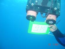
One processing step for the buoy data consists in either eliminating or correcting data corrupted by bio-fouling. The growth of various types of marine organisms, such as algae and bacteria, is unavoidable with moored instruments, albeit it is much less severe in the clear offshore waters at BOUSSOLE than it can be, for instance, in turbid coastal environments. The cleaning of the instruments every two weeks (divers), in addition to the use of copper shutters, rings and tape (see below), contribute to maintaining bio-fouling at a very low level. Possible bio-fouling is identified by comparison of the data collected before and after the cleaning operations, which allows either elimination or correction of the corrupted data.
We have managed to essentially get rid of bio-fouling by using the following measures:
- Cleaning of instrumentation by divers every 2 weeks. This is possible by intermingling two cleaning programs each at a monthly frequency. The first one is operated from the R/V Tethys-II at the occasion of the regular monthly servicing cruises, and the second one is operated by a private company, in between the regular monthly cruises.
- Installation of anti-fouling devices:
- Copper face plate on the backscattering meter.
- Copper face plate + wiper and copper shutters on fluorometers.
- Copper rings around windows of the transmissometers and copper tape on the instrument housings.
- Copper tape on the instrument housings for the 7-bands radiometers.
- Copper shutter and copper tape on the instrument housings for the hyper-spectral radiometers.
Pictures of these devices are provided below.

|
|

|
Copper face plate of the Hobilabs’ Hydroscat-2 backscattering meter |
Copper rings around the emission and reception windows of the Wetlabs C-star beam transmissometers |
Copper tape on the housings of the Wetlabs C-star beam transmissometers |
|
|
|
Copper face plate and copper shutter including a wiper for the Wetlabs Eco-FLNTU fluorometers (shutter closed) |
Copper face plate and copper shutter including a wiper for the Wetlabs Eco-FLNTU fluorometers (shutter opened, measuring) |
Copper tape on the instruments’ housings for the Satlantic 7-band OCR-OCI/200 radiometers |

|
|
|
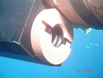
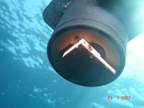
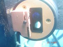
Copper tape on the instruments’ housings and bio-shutter (Satlantic Hyperspectral radiometers) |
|
|
|
| HPLC
analyses |
Sample collection
Seawater samples were collected from Niskin
bottles and filtered through 25 mm GF/F Whatman filters
(0.7 µm porosity). In most cases 2.8 litres
were filtered for each sample and the filters were
placed in Petri slides, wrapped in aluminium
and stored first in liquid nitrogen on board then
in a -80°C freezer in the lab.
Extraction procedure
Each filter is placed in 3 mL of methanol
(HPLC grade) containing an internal standard*.
After 30 minutes at -20°C the filters are disrupted
by ultrasonication using an ultrasonic probe and
returned to the freezer. Another 30 minutes later,
the sample is clarified through a 25 mm GF/C Whatman filter
(1.2 µm porosity). The filtrate is finally
stored at -20°C until analysis (within 24 hours).
HPLC analysis
All parts of the HPLC system at the LOV
are Agilent Technologies products:
- A degasser
(1100 model);
- A binary pump (1100
model);
- An autosampler6 (1100
model) with temperature control (4oC) and automatic
injection (Rheodyne valve) for mixing the sample
with the ammonium acetate (1N) buffer;
- A diode array
detector (1100 model) with measurements at
440nm (for carotenoids), 667nm (for chlorophylls
and degradation products) and 222nm (for Vitamin
E Acetate internal standard); and
- A fluorescence detector
with excitation and emission wavelengths respectively
at 417 and 670nm.
Column temperature is maintained
at 25oC and the injection volume
is 200 μL. The analytical method is based on a gradient separation
between a methanol:ammonium acetate (70:30) mixture
and a 100% methanol solution, comparable to that
described by Vidussi et al. (2000), but with a few
differences allowing for improvement of sensitivity
and peak resolution. Modifications to this method
to separate certain peaks and increase sensitivity
included a) a flow rate of 0.5mLmin-1, and b) a reversed
phase chromatographic C8 column with a 3mm internal
diameter (Hypersil MOS 3μm). The gradient used is
presented in Table 3.
The different pigments that are quantitated are
presented in Table 4. An example of a chromatogram
is shown in Fig. 14.
Back
to top
Pigment
(in order of retention time) |
Detection
wavelength |
Observations |
1. Chlorophyll
c3 |
440 |
|
2. Chlorophyllide
a |
667 |
coelution
with chlc1+c2 |
3. Chlorophyll
c1+c2 |
440 |
|
4. Phaeophorbide |
667 |
coelution
with peridinin |
5. Peridinin |
440 |
|
6. 19’-butanoyloxyfucoxanthin |
440 |
|
7. Fucoxanthin |
440 |
|
8. 19’-hexanoyloxyfucoxanthin |
440 |
|
9. Neoxanthin
+ violaxanthin |
440 |
coelution |
10. Diadinoxanthin |
440 |
|
11. Alloxanthin |
440 |
|
12. Diatoxanthin |
440 |
|
13. Zeaxanthin |
440 |
|
14. Lutein |
440 |
|
15. Non-polar
chlorophyll c1 |
440 |
|
16. Total chlorophyll
b = chlorophyll b + divinyl chlorophyll b |
440,
667 |
coelution |
17. Crocoxanthin |
440 |
|
18. Divinyl chlorophyll
a |
440 |
|
19. Chlorophyll
a = chlorophyll a + allomers + epimers |
440,
667 |
|
20. Non polar
chlorophyll c2 |
440 |
|
21. Carotenes
= α-caroten + β-caroten |
440 |
coelution |
22. Phaeophytin
a |
667 |
|
Table 7.2: **Replace
with new Table 4. The list of pigments detected by
HPLC at the LOV, their detection wavelengths, and
their possible coelution with another pigment. The
variable forms, which are used to indicate the concentration
of the pigment or pigment association, are patterned
after the nomenclature established by the SCOR Working
Group 78 (Jeffrey et al. 1997). Abbreviated forms
for the pigments are shown in parentheses.
Example
of a chromatogram containing all major pigments from
a surface sample at the BOUSSOLE site in April 2003.
Numbers refer to pigment names in Table 4.
Back
to top
Calibration
Response factors for 8 pigment standards provided
by DHI (International Agency for C14 determination,
Denmark) are determined by spectrophotometry (Perkin
Elmer) followed by HPLC analysis:
- Peridinin,
- 19’-Butanoyloxyfucoxanthin,
- Fucoxanthin,
- 19’-Hexanoyloxyfucoxanthin,
- Alloxanthin,
- Zeaxanthin,
- Chlorophyll b,
- Chlorophyll a.
These response factors are then derived to compute
the specific extinction coefficients of these 8
major pigments for the HPLC system.
Specific extinction coefficients for divinyl chlorophyll a and
divinyl chlorophyll b are computed knowing:
- the specific extinction coefficients of chlorophyll a and
chlorophyll b;
- the measurement of the absorption of chlorophyll a and
divinyl chlorophyll a (or chlorophyll b and
divinyl chlorophyll b) at 440 nm when
the spectra of both pigments are normalized at
their red maxima; and
- that both pigments are considered to have the
same molar absorption coefficient at this red
maxima.
For the remaining pigments, their specific extinction
coefficients were either derived from previous
calibrations or from the literature (Jeffrey et
al., 1997).
Quantification
The Agilent Technologies Chemstation software
is used for conducting the analysis as well as for
post-analysis processing. This includes peak integration
and spectral identification. Peak identification
is manually verified by retention time comparison
and observation of the absorption spectra. Quantification
is based on peak area related to the specific extinction
coefficient and concentrations are given in milligrams
per cubic meter. When two pigments tend to co-elute,
their identification is first done spectrally then
they are summed, e.g., chlorophyll c1+c2,
or total chlorophyll b (chlorophyll b plus
divinyl chlorophyll b).
Validation
A
solution of methanol containing the internal standard
is injected every 12 samples during the analytical
sequence. The average of these control analyses provides
the reference peak area for the internal standard.
The standard deviation of these analyses provides
information about the precision as well as the stability
of the instrument during the analytical sequence.
Total chlorophyll a values are compared to the fluorescence
signal from CTD bottle data in order to detect possible
inaccuracies. Total chlorophyll a values are also
compared to particulate absorption measurements which
have been carried out on the same filters just before
pigment extraction (Sect. 7.2).
Method
performance
This HPLC analytical method has
proved to be particularly sensitive, with
detection limits of approximately 0.001 mgm-3
and a good resolution between divinyl chlorophyll
a and chlorophyll a which allow it to be
particularly adapted to the oligotrophic
waters of the Mediterranean.
The precision of the method is generally
characterized by a variation coefficient
between 0.3-1.0%. Furthermore, two international
intercomparison exercises (SeaHARRE-1 (Hooker
et al. 2000) and SeaHARRE-2) have demonstrated
that the LOV produces satisfactory results
for the analysis of chlorophyll a and accessory
pigments in seawater samples from different
concentration regimes.
-----------------------------------------
*Samples
before March 2003 were analysed with trans-β-apo-8’-carotenal as
internal standard then replaced with Vitamin
E Acetate.
Back
to top |
| Filter
pad absorption |
Laboratory
analyses
The protocol for the analysis of spectral absorption coefficients of particulates
is based on those recommended in chapter 15 of the NASA Ocean Optics Protocols
for Satellite Ocean Color Sensor Validation paper (Mitchell et al, 2002).
Sampling is performed in the same way as for the
HPLC pigments as described in Sect. 8.1 where
the seawater samples are collected from Niskin bottles
and filtered through 25mm GF/F Whatman filters (0.7
porosity). In most cases 2.8L are filtered for each
sample and the filters placed in Petri slides, wrapped
in aluminium and stored first in liquid nitrogen
on board then in a -80oC freezer in the laboratory.
The sample filters used for the analysis are also
used afterwards for HPLC analysis. This method has
been tested to ensure that using the same filter
for the two methods does not compromise either measure.
The spectrophotometer used is the Perkin Elmer
Lambda 19 (L19) Dual Path Spectrometer with an integrating
sphere compartment attached. The instrument scan
range is set from 750 to 350nm with a scan interval
of 1nm. After a 1h warm-up period, the machine is
ready to use.
The samples are taken out of the -80oC freezer
and stored temporarily in an ice-cooled cold box.
Each sample, in its petri dish, is then placed in
a dark box on the bench to defrost for 5min. This
defrosting period is kept to a minimum because the
pigment composition once thawed becomes susceptible
to degradation which could affect the analyses, particularly
the HPLC.
The L19, being a dual path spectrometer, has a
slot for a reference material and another for the
sample. These slots are actually the outer walls
of the integrating sphere at the two positions where
the two beams enter the sphere. For the reference
path, rather than use a blank filter, which can create
variations in the spectra attributable to differences
in the level of moistness of the filter, the pathway
is left open (without any filter blank) thus using
an air blank. In the sample material slot, a blank
GF/F filter is used. This blank has been soaked in
distilled water for 12h and had excess water drained
off before being placed in the sample slot.
An autozero is performed with the blank filter
in the sample path and the reference path open, which
sets the absorbency values measured at each wavelength
to zero. As a verification of this and to provide
a baseline, the blank is then scanned to measure
absorbency. The spectra produced from this should
be flat and close to zero (within 0.005). If this
is not the case, the autozero is repeated and the
blanks scanned again.
Once satisfactory baselines have been achieved,
the sample filters can then be scanned. For baselines
and samples, each filter, scanned twice, should result
in two similar replicates. If replicates do not match
well, the filter position should be checked and the
sample scanned again. Drying of the filter between
replicates may cause some vertical offsetting. This
is still acceptable if the spectral shape for each
replicate is similar.
The spectra for each sample are saved as a file
in American Standard Code for Information Interchange
(ASCII) format with two columns: wavelength and absorbency.
The mean of the absorbency values of replicates for
each sample is calculated and any offset from zero
removed by subtracting the absorbency value at 750nm
from the whole spectrum.
Data postprocessing
The optical densities are then corrected for any nonzero signal in the NIR
(750nm), and transformed into absorption coefficients by accounting for the
so-called β effect. The total particulate absorption spectra are then numerically
decomposed into a phytoplankton and a detritus absorption spectra following
Bricaud and Stramski (1990).
Back
to top |
| Buoy
data pre-processing |
The binary log files
for the instruments connected to the OCP-100s are
converted by Satcon into ASCII format files. Satcon
uses the calibration coefficients and format information
in the calibration (|*.cal|) files, created by Satlantic
during the most recent absolute calibration, to convert
the raw counts to physical units. The compass and
tilt sensor data are converted by Satcon using coefficients
and information in a text definition file (|*.tdf|),
provided by Satlantic. The ASCII files produced by
Satcon are given the file extension |*.dat|.
The Hydroscat log file data are converted to physical
units using HOBI Labs' Hydrosoft software and the
HOBI Labs calibration files and output to (|*.dat|
ASCII) files. There are no valid time values associated
with these files, except the time of file creation
in the filename.
The CTD |*.log| files do not require any pre-treatment
before they are concatenated and merged with the
other instrument data. There is no time data associated
with these files except for the file creation time
in the log file name.
A Matlab processing script removes header lines
from all the ASCII |*.dat| files then, where multiple
files for one day exist, these are concatenated into
a single file for each day and for each instrument.
In order to have a single day file for all the instruments,
the timeframe of the OCP4 file is used as a standard
for each of the other files. Therefore, the number
of rows in the final file is always the same as the
OCP4 file. Two processes are required for integrating
the other instrument files, one for the files that
have their own time stamps already and one for those
that do not. The latter relates to the CTD and hydroscat
files.
Where a time stamp is present for an instrument,
integrating the data time frame for this instrument
into the OCP4 timeframe is performed by finding the
closest time stamp in the OCP4 file which is less
than the time stamp for each line of the file of
interest and within the same 1min sampling period.
For the hydroscat and CTD data, which have no timestamp,
their integration into the OCP4 timescale is performed
using the proportion of each 1min OCP4 sampling period
to the entire day's OCP4 data. The progressive proportions
of each of these sampling period for a day's data
is then used to divide up the day's CTD and hydroscat
data to the same ratio. Once these files are divided
up into theoretical 1min slots, the data lines within
each slot are then distributed evenly across the
true 1min sampling period of the OCP4.
For the seven radiometers ( 1=OCR-2001 and 1=OCI-2001
), a dark correction is performed by subtracting,
from each radiometer data series, the mean data values
collected between the hours of midnight and 0200
hours for each instrument. After processing, general
radiometer health can be assessed for each day by
monitoring these dark values. The dark values for
each instrument are, therefore, saved to a file where
they can be easily checked for changes. The buoy
data after pre-processing is presented as large (approximately
13MB) individual files containing all instrument
data for a single day from midday to midnight.
|
| AOPs
from the SPMR profiles |
The SPMR is a central element in our program. It is
providing reference data against which the data
collected from the buoy can be checked, and it
is providing also the information on the vertical
that is not provided by the buoy surface measurements.
Measurement
suite
What is measured
in the water column is
the upwelling irradiance,
Eu(z, λ), at 13
wavelengths from 412-865nm,
plus the downward irradiance
at the same wavelengths,
Ed(z, λ). The latter is not used
in the computation of the
reflectance.
The above-water downward irradiance, Ed(0+, λ),
0+ indicates a height immediately above the surface),
which is often referred to as Es(λ), is recorded on deck
(at the bow of the ship), again at the same 13 wavelengths.
Corrections
and extrapolations
From the vertical profile of Eu(z, λ),
the upwelling irradiance at null depth, i.e., immediately
below the sea surface,
is obtained as (λ
is omitted for brevity) :

where z is
depth (0- indicates a height immediately
below the surface amd is referred to as the null
depth),  is
the shallowest value of is
the shallowest value of  for
which the tilt is less than 2o, and Ku is
the attenuation coefficient for the upwelling irradiance
computed from the measurements of collected
at different depths between for
which the tilt is less than 2o, and Ku is
the attenuation coefficient for the upwelling irradiance
computed from the measurements of collected
at different depths between  and and  m. m.
Several interpolation procedures designed to derive
the
Eu(0-)
from the vertical profile of have
been tested against true values of Eu(0-) (i.e.,
values directly measured below the sea surface by
installing the radiometer on a floating frame), and
the method that eventually provided the closest values
to the true ones was selected. This experimental
work, which is not further detailed here, is just
mentioned to indicate that the contribution to the
overall uncertainty budget of the extrapolation error
has been minimized and is below 3% across the entire
spectrum.
The above-water reference measurement, Ed(0+) is
corrected to account for the loss of irradiance at
the air-sea interface:

where the mean transmission of the sea surface
for sky and sun irradiance, expressed by , is equal
to 0.957 (3% according to atmospheric turbidity and
sun elevation), and the internal reflectance (accounted
for by , where is ), varies slightly with . With
a mean value of 3% this term is equal to 0.985 (1.5%
if varies between 0-6%). Assuming these two terms
are constant,

where the value of Ed(0+) is
obtained from the first 10s of recording starting
after the release of the SPMR (this corresponds approximately
to the upper 5m of the descent), to which a fit is
adjusted in order to eliminate variations in Ed(0+) that
are only due to the tilt of the SMSR (which is not
installed on a gimbal). This technique provides similar
results as compared to just picking the measurements
taken for tilt angles less than 1o.
Computed parameters
The reflectance R is then
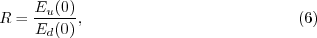
Note that before the
above ratio is formed, the Eu(0-)
is corrected for instrument self shading as per Gordon
and Ding (1992). In this correction, the instrument
radius, the
total absorption coefficient, and the ratio between
direct-sun and diffuse-sky irradiances (rd)
is computed following Gregg and Carder (1990).
Back
to top |
| AOPs
from buoy data |
| To be completed |
| Sun
photometer data |
Numerous methods
have been developed in the past years, which
are dedicated to the retrieval of some kind
of information about aerosol types, usually
particle size distributions, refractive index,
or phase functions from measurements of sky
radiances collected either in the principal
plane, following almucantars or in the solar
aureole (e.g. Santer and Martiny 2001; Dubovik
and King, 2000; Dubovik et al. 2000; Nakajima
et al. 1983; 1996),
A similar method has been developed, which
in addition uses the information provided by
the degree of polarization, as measured at
870nm by the sky photometer. Using this additional
piece of information in principle decreases
the ambiguities.
In order to find the best candidate aerosol
model that allows a reconstruction of the sky
radiances distribution observed in the principal
plane, the method either uses the trial-and-error
principle or a more sophisticated inversion
algorithm based on the use of a neural network.
A radiative transfer code is used in these
inversions, which is based on the successive
orders of scattering method and uses the vector
theory OSOA code (Chami et al. 2001).
As for the neural network, which has the
advantage of allowing fast processing of time
series, and which is able to properly deal
with measurement errors, the important step
is the training. This training has been performed
by using the OSOA radiative transfer code (Deuze
et al. 1989; Chami et al. 2001), and using
aerosol models with varying index of refraction
and a particle size distribution following
a Jünge model. A realistic noise that
accounts for instrumental errors is added on
the synthetic data.
|
|
|
|
|