|
|
QUANTITATIVE DATA SUMMARY |
Initial
results
In the following sections,
sample results are provided essentially to illustrate
the site characteristics.
|
| Summary
tables of the data collected |
|
| Physical
conditions |
The figure below is a time series of the temperature over the first
200 meters of the water column, from July 2001 to
December 2005. The well-known winter mixing and spring
stratification clearly appear, as well as the increase
of the surface temperature from year to year. The
summer of 2003 was one of the warmer recorded over
the last decades in northern Europe, and the signature
of this unusual climate is evident here in the temperature
record. Another noticeable feature appears in winter
of 2005, when the temperature did not reached the
usual 12.9 degrees minimum, which is in principle
a recurrent characteristics of this area where deep
mixing occurs in winter, forming by this way the
deep waters of the western Mediterranean basin.
Time
series (July 2001 – June 2005) of the potential
temperature over the 0-200 meters depth.
Back
to top |
| Phytoplankton
pigments |
Pigment
samples for HPLC analysis have been collected at
about 12 depths between the surface and 200 meters
at the BOUSSOLE site since July 2001. Surface samples
at 5 and 10 meters depth were collected in triplicate.
During certain surveys only surface samples were
taken. In the following section, results from these
analyses over 2 years from July 2001 to July 2003
are briefly described.
Total chlorophyll
a seasonal evolution
During the winter periods the highest values
for TChla have been observed, particularly for the
month of February, when maximum values at the surface
reached 1.34 (in 2002) and 2.44 mg.m-3 (in 2003,
Figure below). In February 2002 the water column appeared
to have undergone strong vertical mixing just before
the survey, with Tchla a concentrations averaging
0.845 mg.m-3 (± 5%), down to 130 meters depth.
March and April are
characterized by the spring bloom in surface waters,
with TChla values reaching 1.23 mg.m-3. In March
2003, a deep chlorophyll maximum (DCM) already began
to form at 50 m.
During summertime, surface
TChla concentrations remain low (0.1 to 0.2 mg.m-3).
However, this trend is
not reflected for deep samples (below 10 m) where
important development of phytoplankton takes place
during the oligotrophic conditions of this Mediterranean
site. The thickness of the DCM at 50 m tends to decrease
towards the end of the summer period.
Autumn marks the transition
between stratified summer conditions and winter turbulence
of the water column, with the progressive increase
of surface TChla concentrations.
TChla
variations between July 2001 and April 2004 for depths < 5
meters (stars) and for depths > 5 meters and < 10
meters (circles). Each point is the average of all
measurements taken during a cruise, and the vertical
bars are the standard deviations within each cruise.
Back
to top
TChla
(diamonds; solid line) and Divinyl Chlorophyll a
(circles, dotted line) 0-200 meters vertical profiles,
and for the dates indicated.
Changes in community structure
Seven carotenoids were partitioned into three phytoplankton size classes and normalized by the sum of the 7 pigments (Vidussi et al, 2001):
- Picophytoplankton, [TChl b] + [Zea];
- Nanophytoplankton, [But] + [Hex] + [Fuco]; and
- Microphytoplankton, [Peri] + [Fuco]
The f igure below presents the variations of these 3 classes between July 2001 and July 2003 at the surface (between 0 and 10 m). Generally, for surface waters, microphytoplankton (characterized by diatoms and dinoflagellates) and nanophytoplankton (characterized by prymnesiophytes and crysophytes) tend to vary in opposition with picophytoplankton (characterized by cyanobacteria at this site). The first are not a dominant class over the studied period, with minimum values in autumn. Nevertheless, at depth microphytoplankton can reach important proportions relative to the other two classes, particularly in spring. Nanophytoplankton is a dominant class in surface waters over most of the year, except during the autumn when picophytoplankton tends to take over. However, the DCM is dominated by nanophytoplankton over the whole summer-autumn period.
The presence of divinyl chlorophyll a, an indicator of prochlorophytes, has generally been observed during autumn at the DCM and even in surface waters during winter convection.
As for the concentrations in chlorophyll a degradation products (Chlorophyllid a and Phaeophorbid a), they were most often below the detection limits of the instrument.
Time
series of average abundances of pico- (diamonds),
nano- (circles) and micro (triangles) phytoplankton
for surface samples (depth < 10 m) between July
2001 and April 2004. Each point is the average over
all measurements taken during a cruise, and the vertical
bars are the standard deviations within each cruise.
Back to top |
| AOPs
from ship operations |
The figure
below (panels a, b and c) show the July 2001- August
2004 time series of the reflectance ratio R(l)/R(560),
for l = 443, 490 and 510. The next two figures show,
for the same time period, the diffuse attenuation
coefficients of the upper layers for the wavelengths
412, 443, 490, 510, 560 and 670 nm. Finally, and the reflectances (R = Eu(0-)/Ed(0-)) for
the same wavelengths.
On these figures, the
open diamonds and the black dots are for the in situ
data (several points per cruises plus the standard
deviation around the mean of these points), the black
triangles are for the HPLC-determined chlorophylla
concentration, the stars are for the AOPs (either
R, ratio of R at two wavelengths or Kd) as computed
through a model that is fed with the in situ chlorophylla
concentration, and the dotted curve is the chlorophylla
concentration that would be derived through satellite
algorithms using the in situ reflectances ratio.
The difference between the big black dots and the
stars, therefore, represents the anomaly of the measured
AOPs as compared to what is predicted by standard
(global) bio-optical models, considering the in situ
chlorophylla concentration.
Similarly, the difference between the stars and
the dotted curve represents the error in the chlorophyll-a
concentration that is obtained when satellite algorithms,
which were derived from global data sets and are
therefore based on average global relationships between
reflectance ratios and the chlorophylla concentration,
are applied to waters with anomalous optical properties.
One striking feature
is the large anomaly of the blue-to-green ratio in
summer of 2001, with lower-than-expected blue-to-green
ratios, as already identified and quantified in Claustre et
al. (2002) for the year 1999 (PROSOPE cruise).
The reason for that anomaly has been attributed to
the presence in the water of desert dust particles,
absorbing in the blue and scattering in the green.
This anomaly is however less important during the
summer of 2002, and it is vanishing during the summer
of 2003. The transient character of this anomaly
has to be confirmed (for instance with the up coming
data for the summer of 2004). The transient character
of this anomaly has to be confirmed.
Examining the diffuse
attenuation coefficients reveals
that their values in the summer of 2001 are largely
above the modeled values across the entire spectrum,
at least from 412-560nm, and that this difference
is disappearing in summer of 2003. Because is largely
determined by the absorption properties of the medium,
these observations mean that an excess absorption
exists at all wavelengths in the July to September
period in 2001.
The same feature does
not appear in the reflectances,
which are lower than the modeled values in the blue,
again during summer of 2001, yet greater than the
modeled values in the green. Because is, to the first
order, proportional to backscattering and inversely
proportional to absorption, these observation confirm
the presence of an excess backscattering in the green
part of the spectrum. Again, the transient nature
of this anomaly remains to be explained.
Another anomaly is observed
in February 2003, which is now in the opposite direction
as compared to the summer anomaly, with larger-than-expected
blue-green ratios. During the February 2003 cruise,
the chlorophylla concentration was as large as 2mg m-3.
The reason for this behavior might be in the low
scattering coefficients that are typical of a fresh
phytoplankton bloom, where the proportion of large
healthy cells characterized by a low backscattering
efficiency is high, and the contribution of small
detritus is low.
Back
to top
Times
series (July 2001 – August 2004) of the reflectance
ratio R(443)/R(560). The open diamonds are for the in
situ data (several points per cruises plus the
standard deviation around the mean of these points),
and the black circles are the average of these data
over each cruise. The black triangles are for the
HPLC-determined chlorophyll-a concentration, the
stars are for the reflectance ratio as computed through
a model that is fed with the in situ chlorophyll-a
concentration (Morel and Maritorena, 2001), and the
dotted curve is the chlorophyll-a concentration that
would be derived through “satellite algorithms” using
the in situ reflectances ratio.
 |
Times
series (July 2001 – August 2004) of the diffuse
attenuation coefficients Kd(412), Kd (490) and Kd
(560). The open diamonds are for the in situ data
(several points per cruises plus the standard deviation
around the mean of these points), and the black circles
are the average of these data over each cruise. The
black triangles are for the HPLC-determined chlorophyll-a
concentration, the stars are for Kd as computed through
a model that is fed with the in situ chlorophyll-a
concentration (Morel and Maritorena, 2001).
Back
to top
 |
Times
series (July 2001 – August 2004) of the irradiance reflectances
R(412), R(490) and R(560). The open diamonds are
for the in situ data (several points per
cruises plus the standard deviation around the mean
of these points), and the black circles are the average
of these data over each cruise. The black triangles
are for the HPLC-determined chlorophyll-a concentration,
the stars are for R as computed through a model that
is fed with the in situ chlorophyll-a concentration
(Morel and Maritorena, 2001).
Back to top
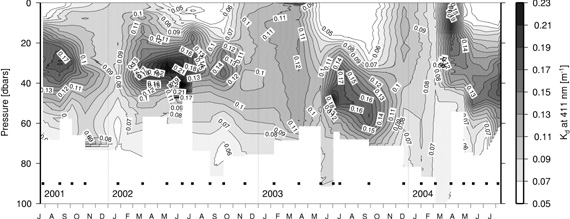
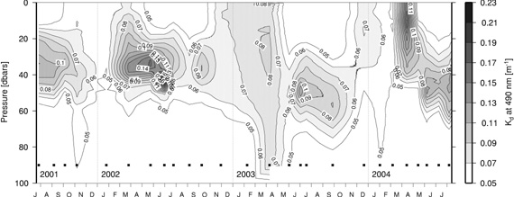
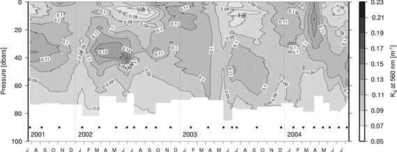
The figure below shows the seasonal and
interannual evolution of the diffuse attenuation
coefficient for wavelengths 412, 490 and 560 nm.
The time series was established from 3 years of measurements
carried out monthly (approximately) from the ships.
This parameter is largely determined by the absorption
coefficient, and it is thus a good indicator of the
concentration of phytoplankton and associated colored
dissolved substances. The seasonal cycle appears
very clearly, in particular in 2003 and 2004: it
starts with an intense mixing of water in winter
(maximum in February, with almost homogeneous properties
and weak ), continues with the start of the spring
bloom in March-April, then evolves gradually to the
oligotrophy, which is maximum around September, and
which is characterized by a maximum of attenuation
at about 50 meters, corresponding to the deep chlorophyll
maximum (DCM). For chlorophyll concentrations lower
than 0.1mgm at the surface at this period, the global
statistical relationships (cf Morel and Berthon,
1989) predict a DCM at about 100 meters. Its development
at a lower depth at the BOUSSOLE site is due to the
situation of this site in the center of a cyclonic
circulation, generating a ôdomeö structure
maintained by significant vertical advection.
The interannual variability observed here for seems
directly related to the changes of the physical framework.
Indeed, the depth of the DCM seems to increase by
2001 to 2004, at the same time as the winter mixing
seems to intensify and the spring bloom being more
intense. The oligotrophic layer of water characterized
by low values of in summer is deeper in 2003 than
in 2001 and 2002. An intense mixing in winter on
the one hand brings more nutrients to the surface,
supporting a stronger bloom, and, on the other hand,
more efficiently eliminates the colored dissolved
substances accumulated at the surface during summer
(phenomenon already shown for dissolved organic carbon;
Copin-Mont‰gut and Avril, 1993; Avril, 2002).
This could explain the changes observed in the "anomalies" of
the marine reflectance (cf. above).
However, the interannual variability of the spring
bloom is somewhat distorted here by an insufficient
sampling in spring 2002 and 2003 (bad weather). Consequently,
it will probably be necessary to rebuild part of
the record by using the vertical profiles of the
pigments and the values derived from the satellites,
coupled with the relationships Chl - that will be
established from the existing data.
Time series of the
vertical distribution of the diffuse attenuation
coefficient at 412 (top), 490 (middle) and 560 (bottom)
nm (derived from SPMR’ Ed vertical profiles).
Red bars indicate the time of the ship sampling.
Units are m-1.
Back to top |
| IOPs
from ship operations |
An annual cycle
of the particulate absorption coefficients at 440
nm is shown below, where the different curves
are for total particles ( ap,
directly measured on filtered samples), and both
the phytoplankton and detrital particles, ( aφ and ad,
respectively). The latter are derived through a numerical
decomposition ( Bricaud and Stramski, 1990) as presented
in Sect. 7.2.
An important feature here is the high
contribution of the absorption by detrital particles,
at least 50% of the total particulate absorption,
from about end of June to the beginning of September.
Time series (2003)
of the absorption coefficients at 440 nm for total
particles (circles), phytoplankton (stars) and detritus
(triangles). The absorption coefficient of phytoplankton
at 676 nm is also shown (diamonds). Top : linear
scale. Bottom : log scale, in order to zoom on the
summer values.
Back to top
The f igure below shows examples of the absorption spectra by particles, either for the total particles or for the phytoplankton or detritus only. The dominant role of phytoplankton in the absorption budget during the spring bloom clearly appears, as well as the progressive increase of that part of absorption that is due to detritus in summer. The exact cause of the background absorption in the UV that clearly appears when absorption decreases at other wavelengths (see the summer spectrum) remains to be identified.
Spectra of the absorption
coefficient of particles at 5 meters (total : solid
curve, phytoplankton : dotted curve, and detritus
: dashed curve), as determined on filtered samples
(method described in section 7.2). Samples collected
in 2003, for the dates indicated.
The figure below shows examples of the total attenuation, scattering and absorption coefficients for the surface (0-10m) layer. One can just mention the clear identification of the absorption features on the scattering spectrum, and the change in its slope from spring to summer (increasing slope in summer corresponding to the large contribution of detritus as compared to phytoplankton themselves).
Spectra of the total
attenuation (circles), absorption (diamonds) and
scattering (stars) coefficients, at the four months
indicated, and for the surface layer (mean from the
surface to a 10 meters depth). Values determined in
situ with the AC9.
The figure below illustrates the richness of the information provided by the IOPs, when compared to modeled values. What is shown here is that a careful analysis of these properties on the one hand confirm what is seen on the AOPs (closure), and, on the other hand, provides clues for the understanding of the causes of variation in these AOPs versus IOPs relationships.
Total scattering coefficient
at 550 nm as a function of the chlorophyll concentration.
Black diamonds : values determined in situ (AC9).
Solid and dashed lines: b(550) as computed from Loisel
and Morel (1998), and a factor of two around the
model values.
Back to top
|
| AOPs
from buoy data |
The figure below shows the data collected
during the deployment of the buoy in March-April
of 2004.
~30-day (11 March – 7
April, 2004) buoy time series of the phytoplankton
fluorescence (top, dotted curve), beam attenuation
coefficient at 660 nm (top, solid curve), R(443)
(bottom, solid curve) and R(560) (bottom, dotted
curve). The vertical dotted bar indicates solar
noon.
Back to top
|
| Sun
photometer data |
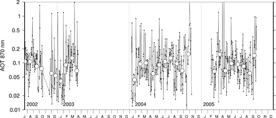
The figure below simply aims at illustrating
the overall data set that has been collected
up to now at the Cap Ferrat sun photometer site.
What is shown is the aerosol optical thickness
as derived by the AERONET project through their
standard procedures.
Time
series of the aerosol optical thickness (AOT at 870 nm) at the Villefranche
Cap Ferrat AERONET site (see at http://aeronet.gsfc.nasa.gov), from July of 2002 to October of 2005. Empty circles are monthly averages.
Back to top
Next, examples are shown that illustrate the capability of the inversion method specifically developed in the frame of BOUSSOLE, which is based on ground-based data to get aerosol optical properties.
For this illustration, we have chosen days corresponding to MERIS overpasses. Results are presented in the figure below for sequences of principal planes corresponding to high solar zenith angles (typically above 70) to better cover the backscattering region of measurements and to include the scattering angle of 150. The accompanying table presents the values of the retrieved refractive index for these sequences. The agreement between measurements and predictions is good especially in the backward direction for sky radiances.
The degree of polarization is also accurately retrieved especially at 90. which is of main interest for the analysis of particles types. These examples show that by applying our inversion algorithm, we were able to derive some information on the refractive indices of aerosols and so, to get the aerosol phase function. Such information allows to satisfactorily predict the angular distribution of the radiance and degree of polarization. Therefore, it makes sense to think that ground-based measurements can be used for the vicarious calibration of satellite ocean color sensors.
Three examples of the
reconstruction of the sky radiances in the principal plane
and at the three wavelengths indicated (curves, left panels),
as compared to the direct measurements of the sun photometer
(symbols), from which the inversion procedure described in
section 7.6 infer an aerosol type. Right panels : idem, for
the polarization rate at 870 nm.
Aerosol optical properties returned
by the inversion algorithm for three days of measurements.
These parameters were used in the computations presented
in the figure above. We also added the aerosol optical depth at 675
nm and the Angstrom exponent a measured by the AERONET radiometer
and the solar zenith angle.
Date |
Time (UTC) |
qs (°) |
mr-jmi |
ta (675 nm) |
a |
July 11 2002 |
17.36 |
72.34 |
1.44-j0.0049 |
0.0955 |
1.562 |
Sept 07 2002 |
16.27 |
72.79 |
1.41-j0.00001 |
0.1143 |
1.686 |
Sept 26 2002 |
15.67 |
72.82 |
1.51-j0.0090 |
0.0385 |
1.459 |
Back to top
|
|
|
|
|